Fine-Tuning
Module: LLM → Fine-Tuning
Fine-tuning lets you adapt a pre-trained large language model to your own data, task or behavioral target. In OICM, the Fine-Tuning module covers the full path from creating a fine-tuning problem, importing data, picking a base model, choosing a problem type and method, all the way to producing a model artifact that is ready to be deployed.
This page covers four things:
- When to fine-tune — and when not to.
- The end-to-end fine-tuning flow — where the OICM module fits in your overall workflow.
- The fine-tuning taxonomy in OICM — dataset types, problem types, PEFT methods.
- The fine-tuning sub-flow inside OICM — what you actually do on the platform, including memory & execution options.
1. When to fine-tune
Before you start a fine-tuning run, it is worth confirming that fine-tuning is the right tool. Fine-tuning typically pays off when:
- Your base model or production model is too slow or too large for your latency or cost budget, and you want to distill its behavior into a smaller model.
- The model lacks knowledge of your domain (terminology, internal entities, formats).
- You need a specific behavior, style, tone or output format that is fragile to reproduce via prompting.
- You have a narrow, high-volume task (classification, extraction, structured generation) where a smaller fine-tuned model can outperform a larger general one.
Fine-tuning is not the first thing to reach for. We recommend ruling out simpler alternatives first:
- Better prompting: clearer system prompt, structured output instructions.
- Few-shot: a handful of examples in the prompt.
- Retrieval-augmented generation (RAG): when the problem is "the model does not know my facts" rather than "the model does not know how to behave".
If those are not enough, fine-tuning in OICM is the next step.
2. End-to-end fine-tuning flow
The picture below shows the whole journey from spotting the problem to deploying a fine-tuned model. Only the green region happens inside OICM — everything else is your team's responsibility outside the platform.
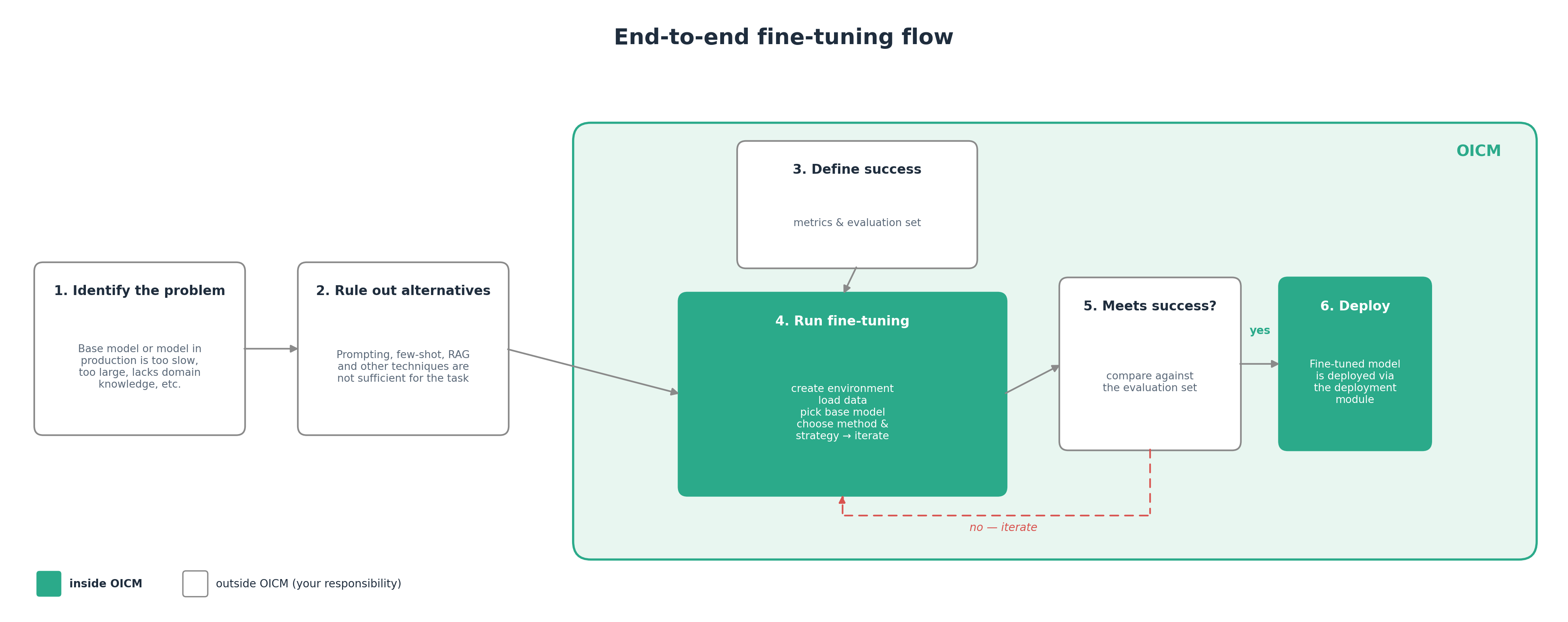
| # | Step | Where | What happens |
|---|---|---|---|
| 1 | Identify the problem | Outside OICM | Your team observes that a base model or model in production does not meet expectations (latency, size, domain coverage, behavior). |
| 2 | Rule out alternatives | Outside OICM | Confirm that prompting, few-shot and RAG are not sufficient for the task. |
| 3 | Define success | Outside OICM | Decide what "good enough" means: pick the metric(s) and prepare an evaluation set that the fine-tuned model must beat. |
| 4 | Run fine-tuning | Inside OICM fine-tuning | Create a problem (task), pick a base model, load data (add data volume), choose a problem type and method while creating the task, run, iterate. Documented below. |
| 5 | Meets success? | Inside OICM fine-tuning | Compare the fine-tuned model against the evaluation set. If it does not meet the criteria — go back to step 4 and iterate. |
| 6 | Deploy | OICM Deployment module | Hand the fine-tuned model off to Deployment to serve real traffic. |
Note
OICM does not impose a success metric or an evaluation set. You define both. The platform helps you reproduce and compare runs against a target you bring in yourself.
3. Fine-tuning taxonomy in OICM
Every fine-tuning run in OICM is defined by three orthogonal choices: the dataset type (the shape of the input data), the problem type (what the run is for), and — for SFT, Alignment and Distillation — the PEFT method (how the parameters get updated).
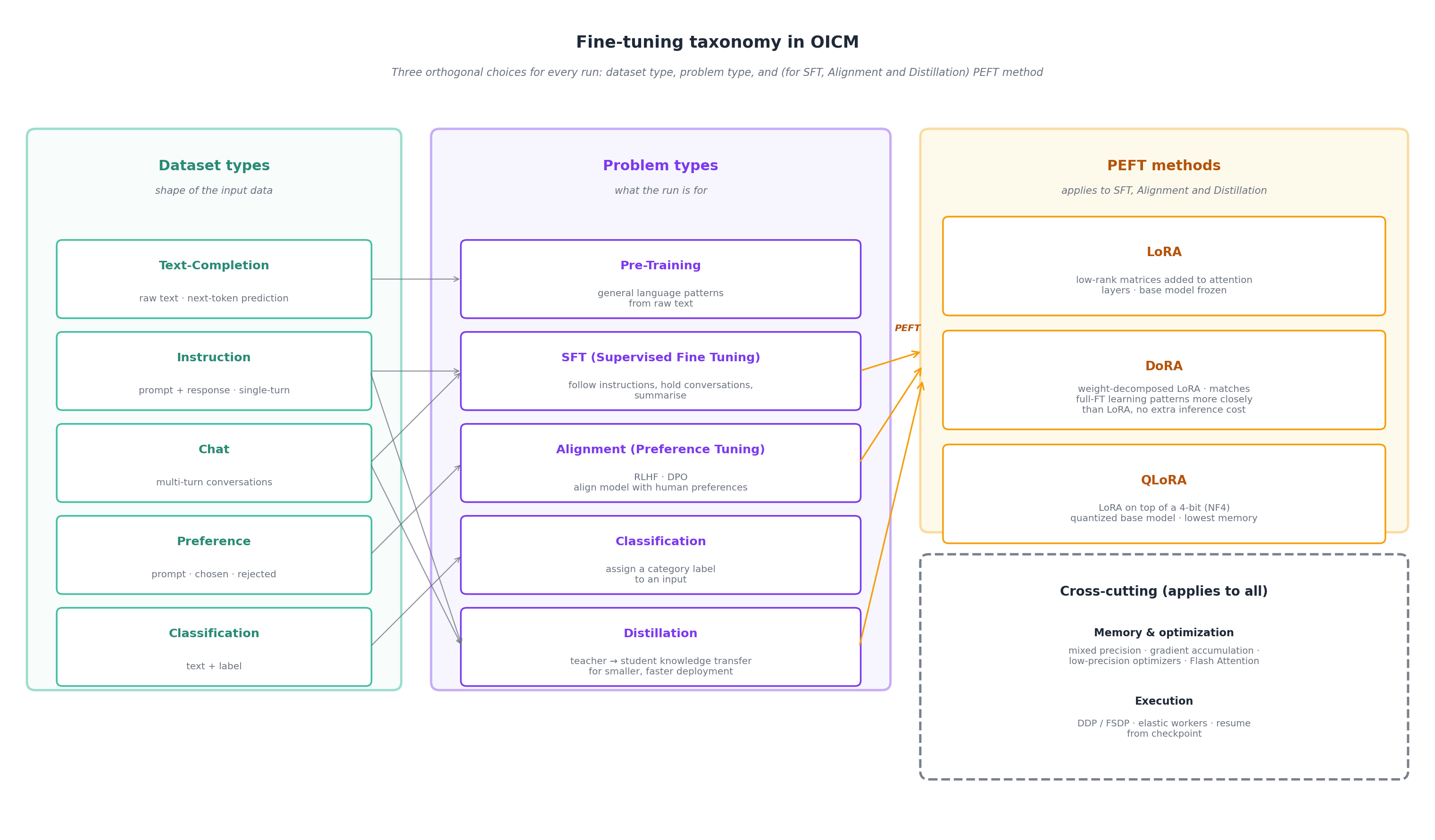
3.1 Dataset types
A dataset type describes the shape of the input data. You bring the dataset into OICM via data volumes (see section 4.2). OICM supports five dataset types:
| Dataset type | Shape | JSONL example |
|---|---|---|
| Text-Completion | Unstructured raw text for next-token prediction. | { "input": "Lorem ipsum raw text 1" } |
| Instruction | Structured single-turn prompt/response pairs (sometimes called question/answer). | { "system": "You are a nice bot", "prompt": "Hello world", "response": "Bye world" } |
| Chat | Multi-turn conversations with system / user / assistant roles. | { "messages": [ {"role":"system","content":"..."}, {"role":"user","content":"..."}, {"role":"assistant","content":"..."} ] } |
| Preference | Ranked responses with chosen and rejected examples for the same prompt. | { "system": "You are a nice bot", "prompt": "...", "chosen": "...", "rejected": "..." } |
| Classification | Text with a categorical label. Schema to be finalized. | { "prompt": "...", "label": "..." } |
Full JSONL examples:
// Chat
{
  "messages": [
    {"role": "system",    "content": "..."},
    {"role": "user",      "content": "..."},
    {"role": "assistant", "content": "..."}
  ]
}
// Preference
{
  "system": "You are a nice bot",
  "prompt": "...",
  "chosen": "...",
  "rejected": "..."
}
Note
If your base model has a chat template baked into its tokenizer, OICM will use it by default and that usually gives the best results. Most instruct and chat models ship with a chat template; most base (non-instruct) models do not. When a tokenizer has no template, OICM falls back to a default template that looks like this:
3.2 Problem types
A problem type defines what the run is for. OICM supports five problem types.
3.2.1 Pre-Training
The model learns general language patterns by predicting the next token in raw text. No structured dataset is required — just continuous text from books, Wikipedia, internal corpora, etc.
- Dataset type: Text-Completion.
3.2.2 SFT — Supervised Fine-Tuning
Fine-tunes a model to follow instructions and hold conversations. Regardless of the dataset, the model is trained as language modeling: auto-regressively, producing one token at a time, conditioned on the preceding tokens. The model structure is not changed; only a chat template is applied to the data. What differs between SFT runs is the shape of the dataset:
- Instruction dataset — single-turn prompt/response pairs.
- Chat dataset — multi-turn, conversational data.
- Dataset types: Instruction or Chat.
Note
SFT supports a few quality-of-life options: excluding the system prompt from loss calculation (masking with -100), and fast tokenizer.
3.2.3 Alignment — Preference Tuning
Aligns model outputs with human preferences using paired chosen/rejected examples. OICM v1.13 supports two alignment methods:
- RLHF — Reinforcement Learning from Human Feedback, through PPO.
- DPO — Direct Preference Optimization.
- Dataset type: Preference.
3.2.4 Classification
Assigns a categorical label to a text input. A classification head is added on top of the base model and trained on labeled examples. Use this when you need a dedicated classifier (sentiment, topic, intent, moderation) rather than a generative model.
- Dataset type: Classification.
3.2.5 Distillation
Knowledge distillation transfers knowledge from a larger, more capable model (the teacher) to a smaller, more efficient model (the student) while adapting the student to a specific task. Useful when you need a compact model that retains most of the teacher's performance but is cheaper to serve, especially in resource-constrained environments such as edge devices.
Components:
- Teacher model — a large pre-trained model already fine-tuned on the target task.
- Student model — a smaller pre-trained model, distilled for the same task.
3.3 PEFT methods (applies to SFT, Alignment and Distillation)
Parameter-Efficient Fine-Tuning (PEFT) targets only a small subset of parameters while the base model stays frozen. PEFT methods make SFT, Alignment and Distillation runs cheaper to run and cheaper to store — many adapters can coexist on top of a single base model. OICM v1.13 supports three PEFT methods:
| Method | What it does | Trade-off |
|---|---|---|
| LoRA | Low-rank matrices are added in parallel to attention layers. The base model is frozen; only the low-rank matrices are trained. | Cheaper and well-supported baseline. Good starting choice for most SFT, Alignment and Distillation tasks. |
| DoRA | Weight-Decomposed LoRA: the pretrained weight is decomposed into a magnitude vector and a directional matrix; LoRA is applied to the directional part, magnitude is fine-tuned directly. | Matches full fine-tuning learning patterns more closely than LoRA and consistently outperforms it on common benchmarks, with no additional inference latency. Recommended as the default replacement for LoRA. |
| QLoRA | The base model is quantized to 4-bit (NF4); standard LoRA adapters are trained on top of the frozen low-bit backbone. | Lowest VRAM footprint. Use when GPU memory is the bottleneck. |
Tip
Start with LoRA on a small base model and a small dataset to validate the pipeline. Switch to DoRA for better quality at the same compute cost. Switch to QLoRA when you hit a memory ceiling.
4. Fine-tuning sub-flow inside OICM
This section walks through the Fine-Tuning module step by step: from creating a fine-tuning task, configuring a run, launching it, monitoring progress, and inspecting results.
4.1 Create a fine-tuning task
In the OICM workspace, open the Fine-Tuning module from the left sidebar. On a workspace where no task exists yet, you will see the empty-state screen with a Create Fine-tuning button.
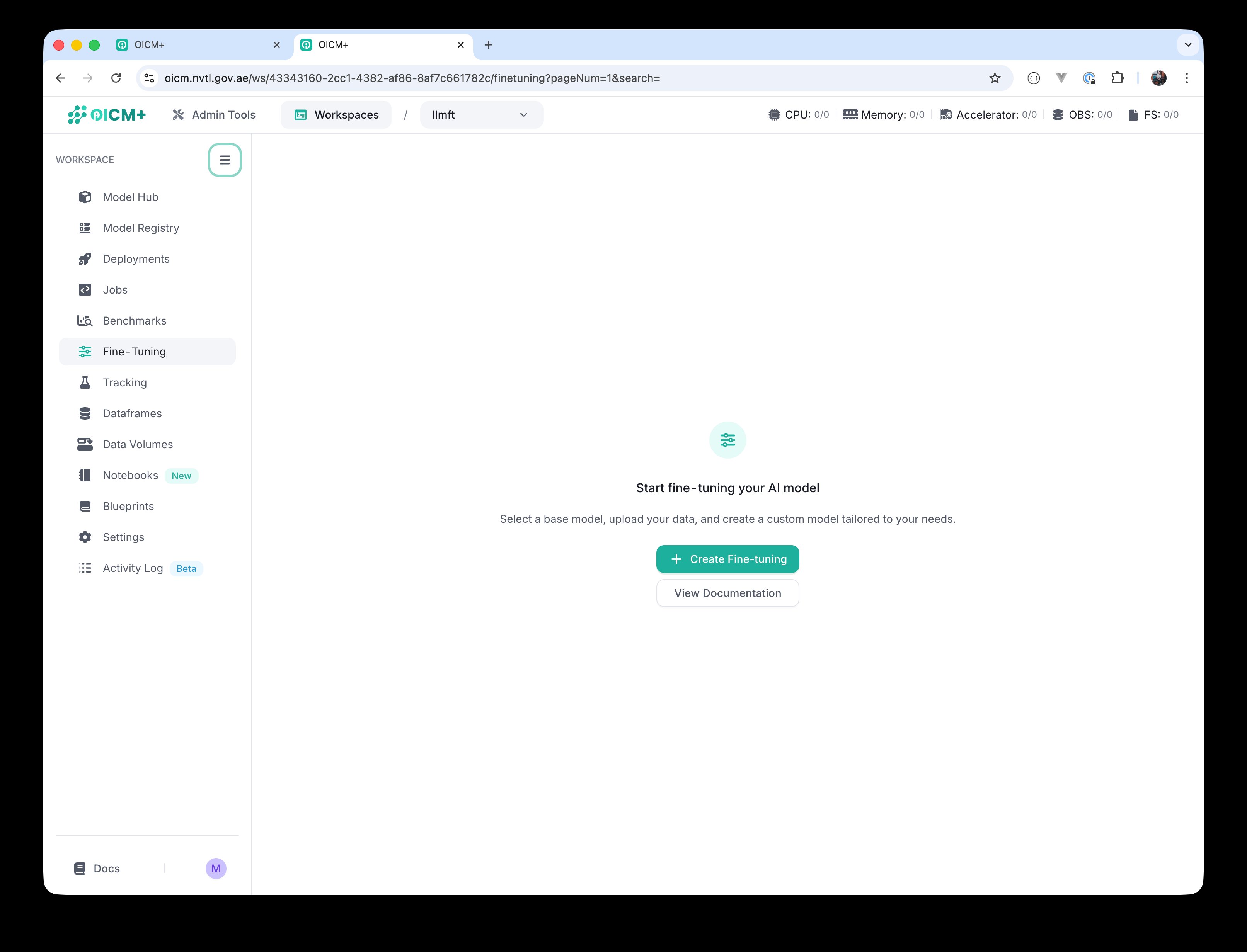 Fine-Tuning module — empty state.
Click Create Fine-tuning to open the Create Fine-tuning Task screen. Fill in:
- Task Name — a unique name that helps you identify and manage this task later (e.g.
sft-0orqwen-dolly-sft). - Task Type — pick one of the six problem types described in section 3.2: Supervised Fine-Tuning, Direct Preference Optimization, Reinforcement Learning with Human Feedback, Classification, Pretraining, or Distillation.
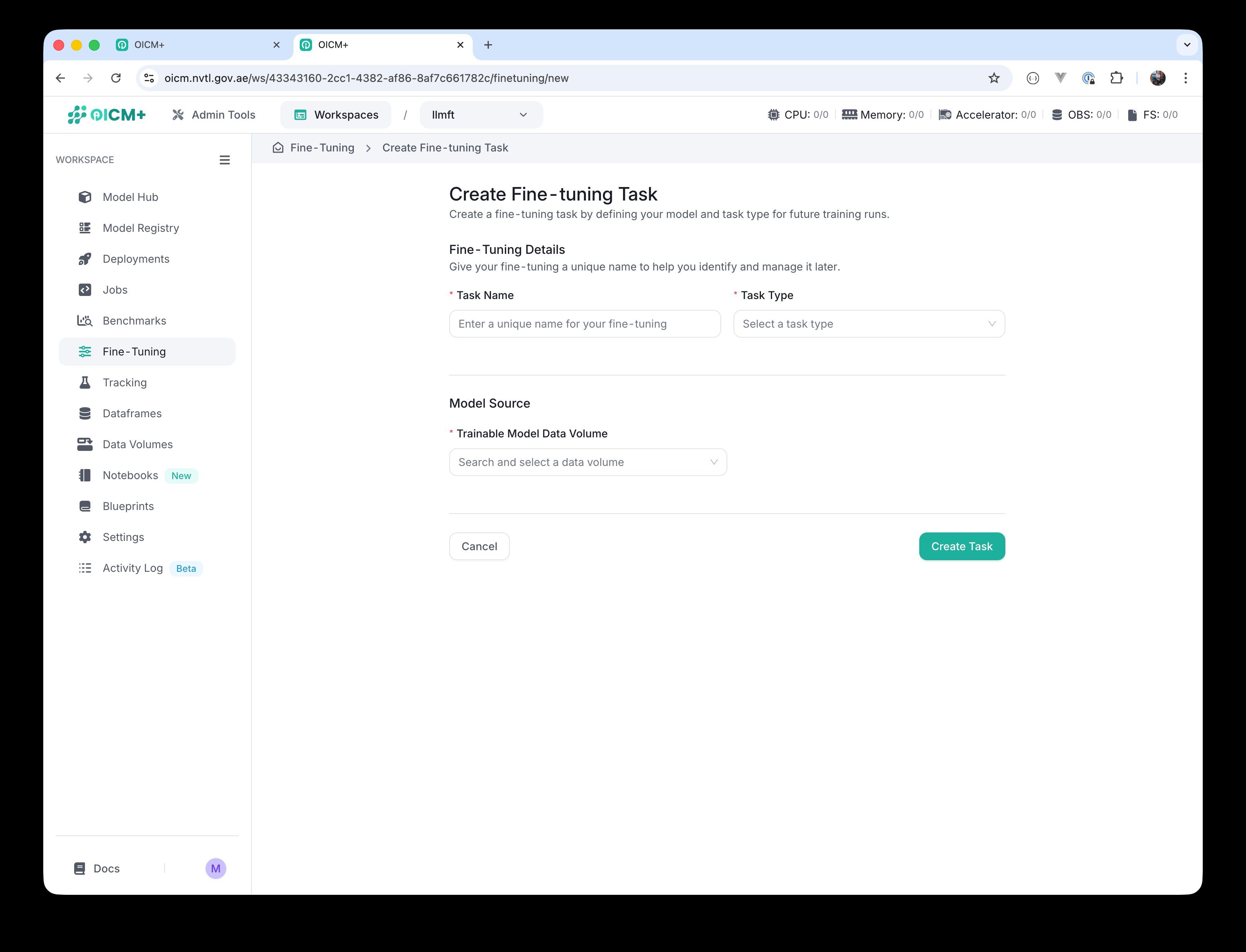 Create Fine-tuning Task — initial form.
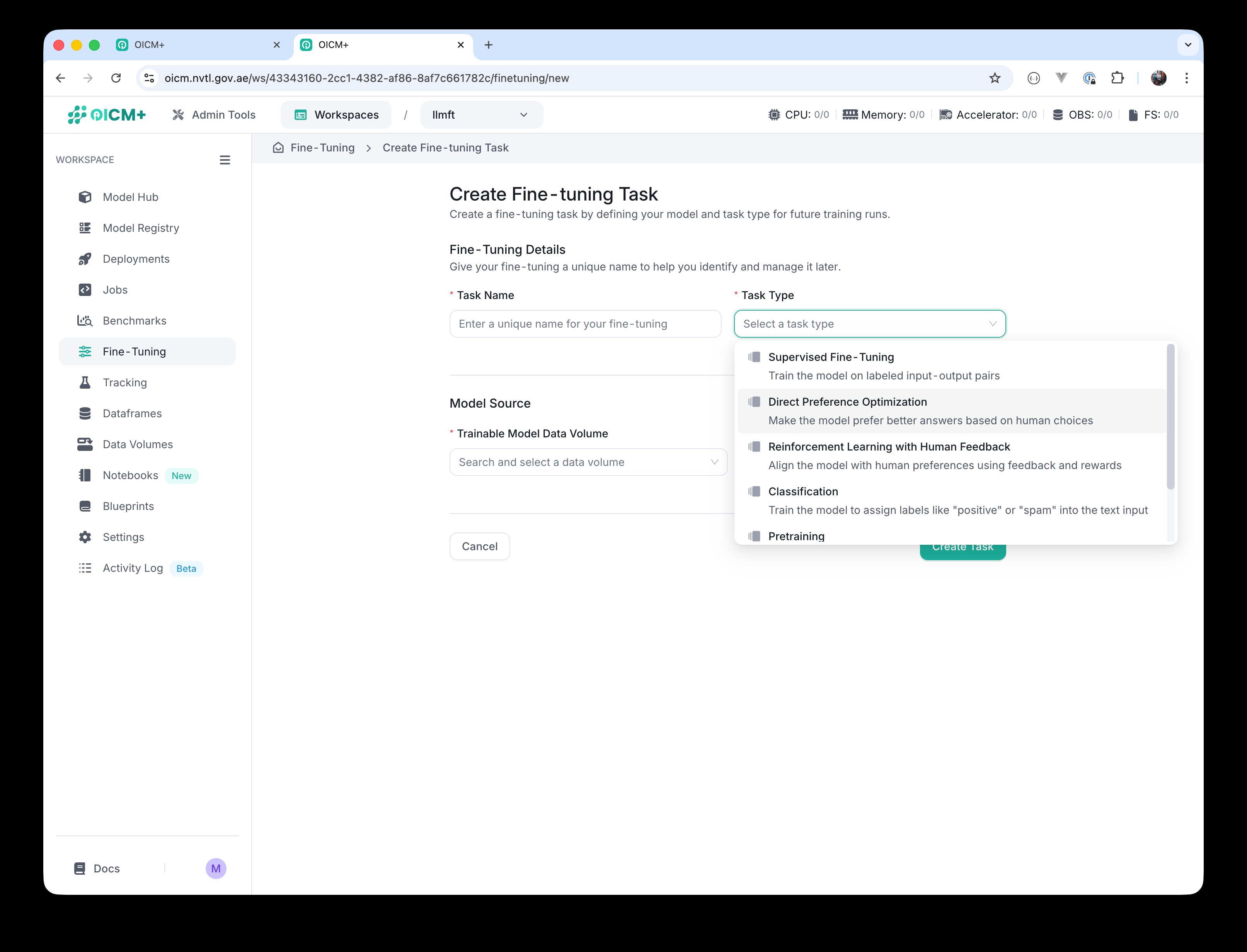 Task Type dropdown — six options corresponding to the problem types in section 3.2.
Model Source — depends on the task type
The Model Source section adapts to the task type you choose:
-
For most task types (Supervised Fine-Tuning, DPO, RLHF, Classification, Pretraining) — one input is required: Trainable Model Data Volume. This is the base model that will be trained.
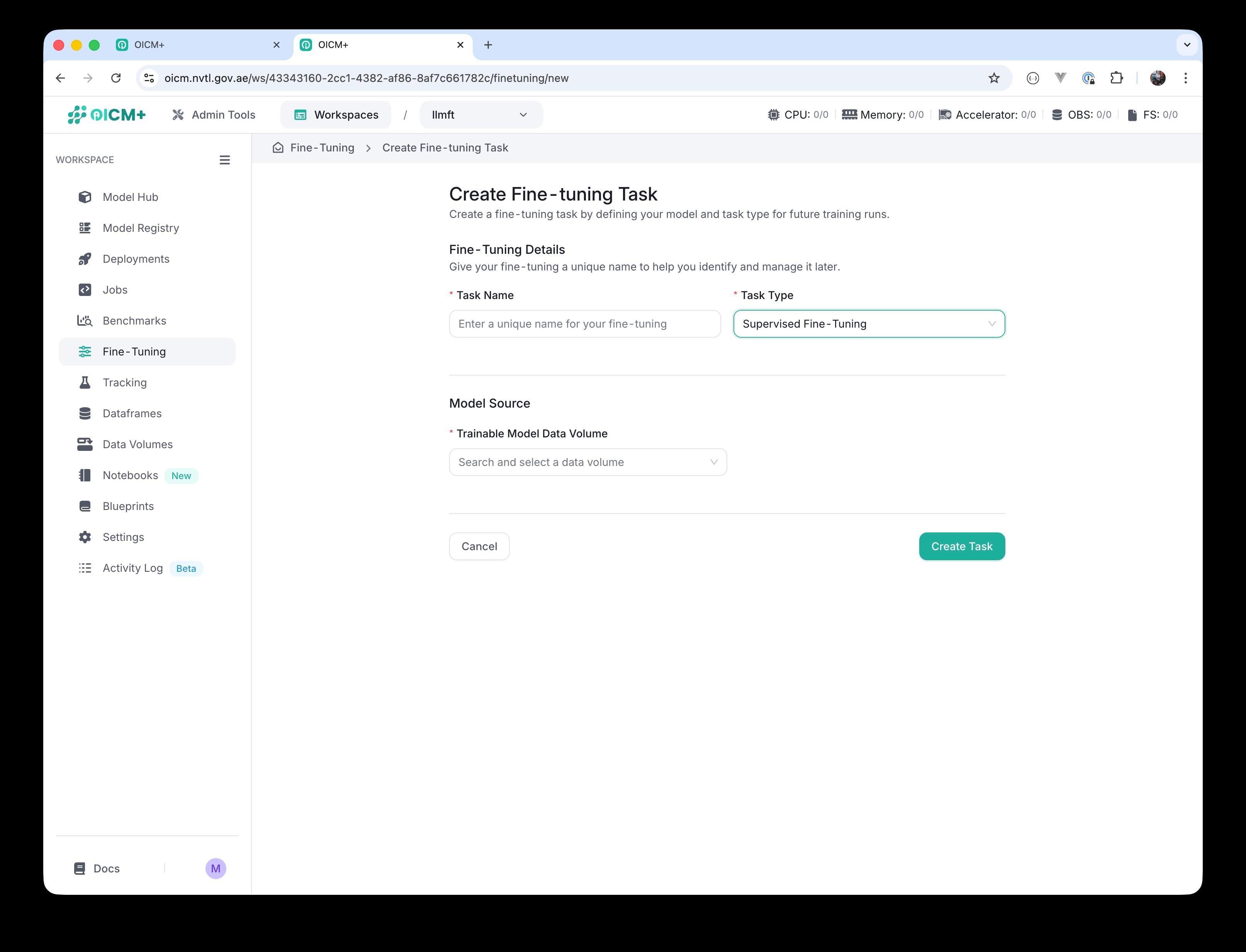 Supervised Fine-Tuning selected — single Trainable Model Data Volume.
 -
For Distillation — two inputs are required: Trainable Model Data Volume (the student model) and Trainer Model Data Volume (the teacher model).
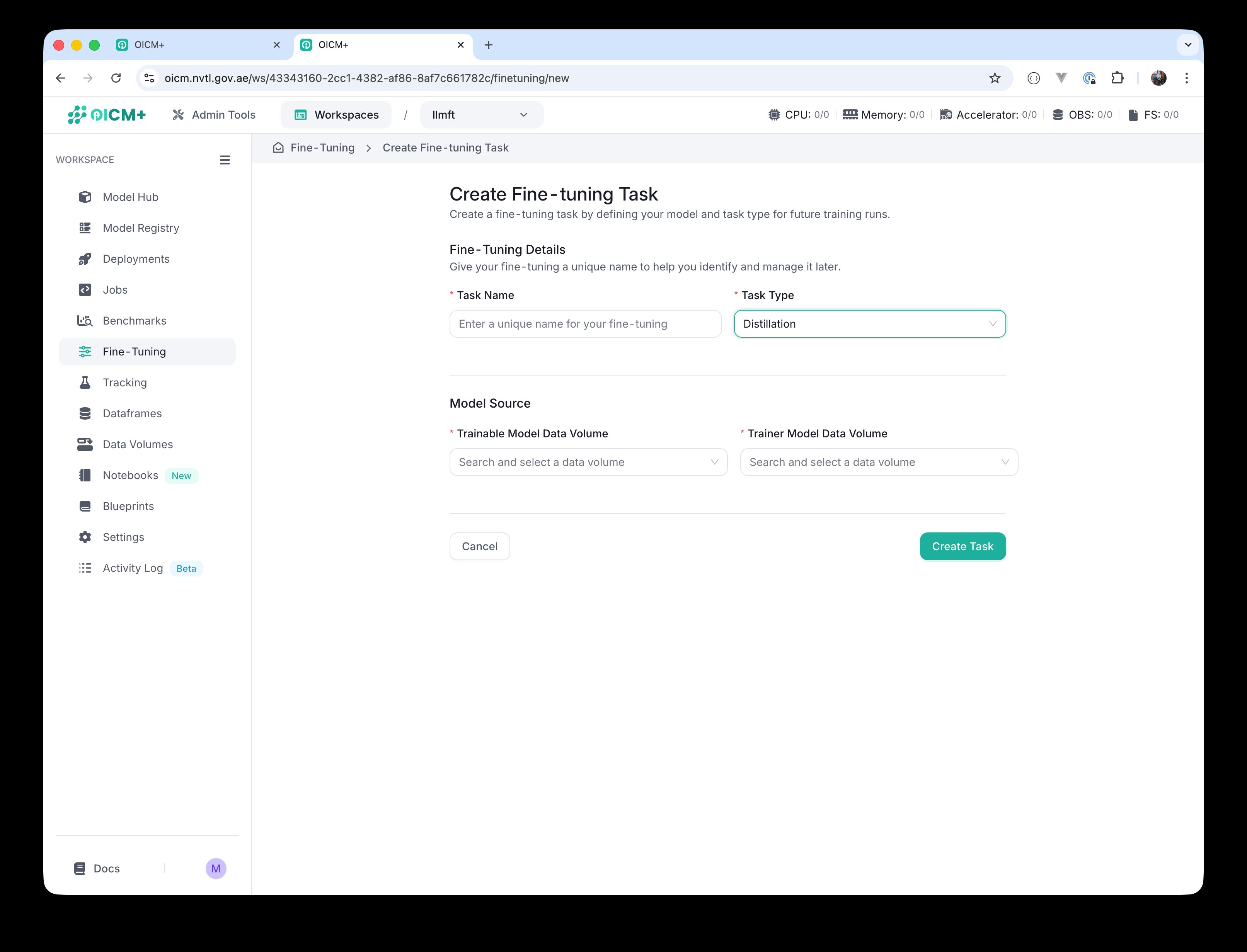 Distillation selected — Trainable (student) and Trainer (teacher) Data Volumes are required.
 Distillation Model Source with both data-volume pickers visible.
Note
The model data volumes referenced here must be prepared in advance in the Data Volumes module. Without an existing data volume containing the base model (and a separate one containing the teacher model for Distillation), you will not be able to complete this step.
Click Create Task to finish task creation. You are now taken to the task overview screen, which shows Task Information (Base Model, Task Type), a Best Performance widget (empty until you have completed runs), and a Create Run button.
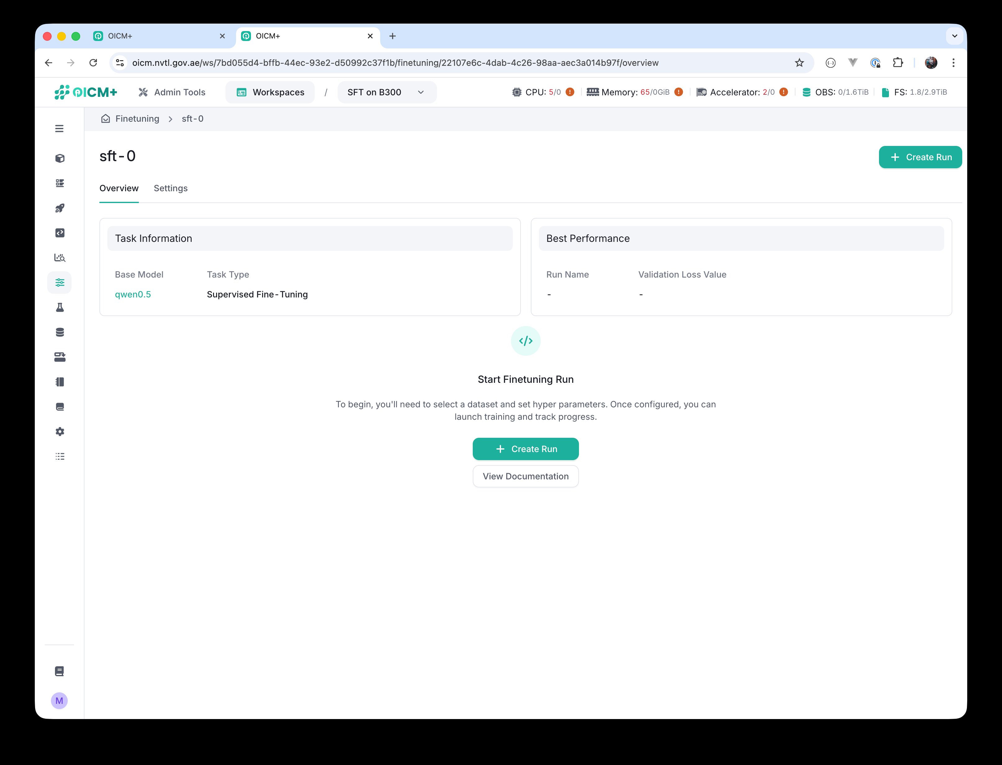 Task overview after creation — ready to create the first run.
4.2 Create a fine-tuning run
On the task overview, click Create Run. The Create Fine-Tuning Run wizard opens with four steps: Run Name, Dataset, Hyperparameters, Resources.
Step 1 — Run Name
Provide a Run Name. You can optionally add a Description to record what makes this run different from others on the same task.
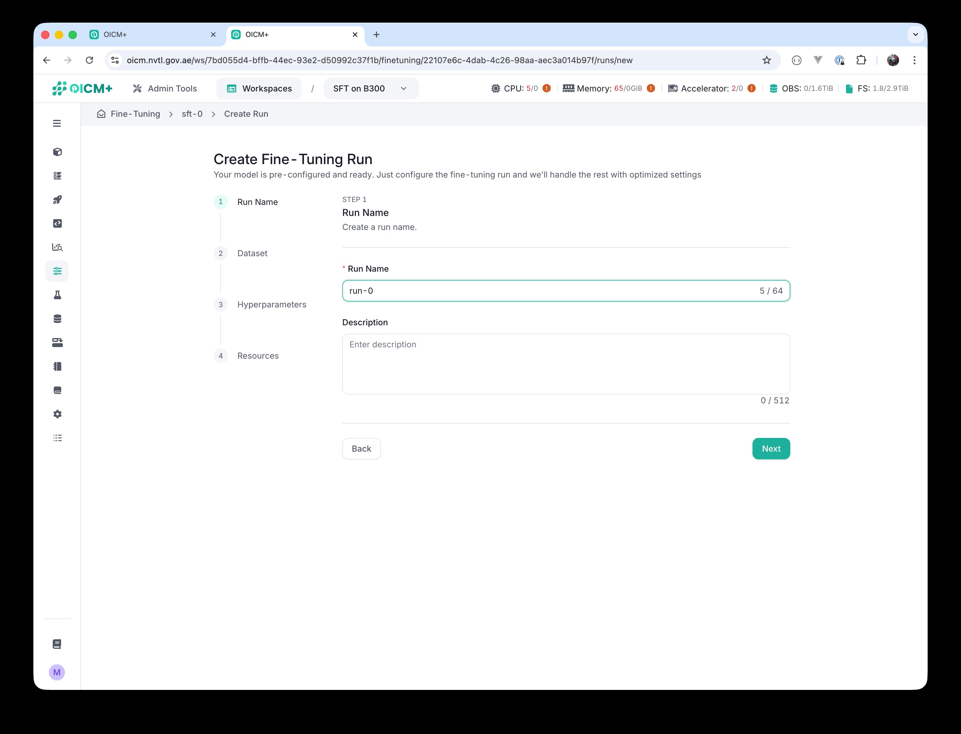 Step 1 — Run Name and optional Description.
Step 2 — Dataset
In the Dataset step, you select the training and validation datasets and map their columns to the fields the fine-tuning task expects.
- Training Dataset: pick a Data Volume from the available data volumes in the workspace, then pick one or more dataset files (typically Parquet) from that volume.
- Column Mapping (training): map the dataset columns to the fields the run needs:
- User Prompt
- Answer
- Conversation ID
- System Prompt
- Validation Dataset: repeat the same selection and column mapping for the validation set. It can come from the same Data Volume as the training set.
Note
Supported file types are CSV, JSON/JSONL and Parquet.
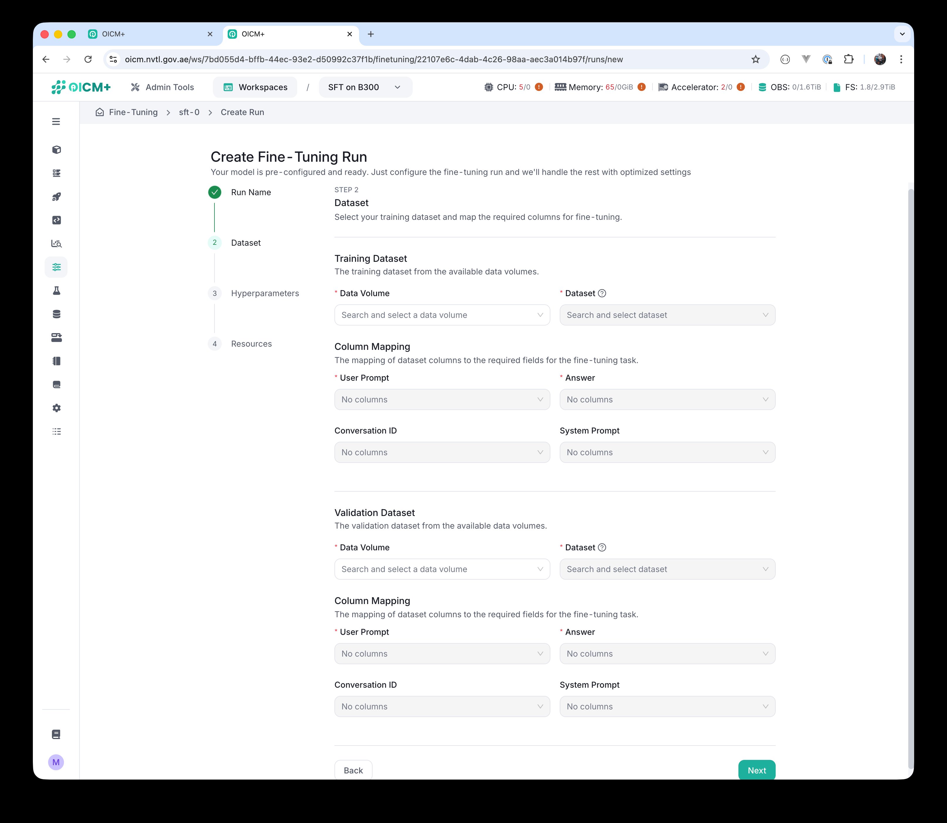 Step 2 — Dataset selection and Column Mapping, empty state.
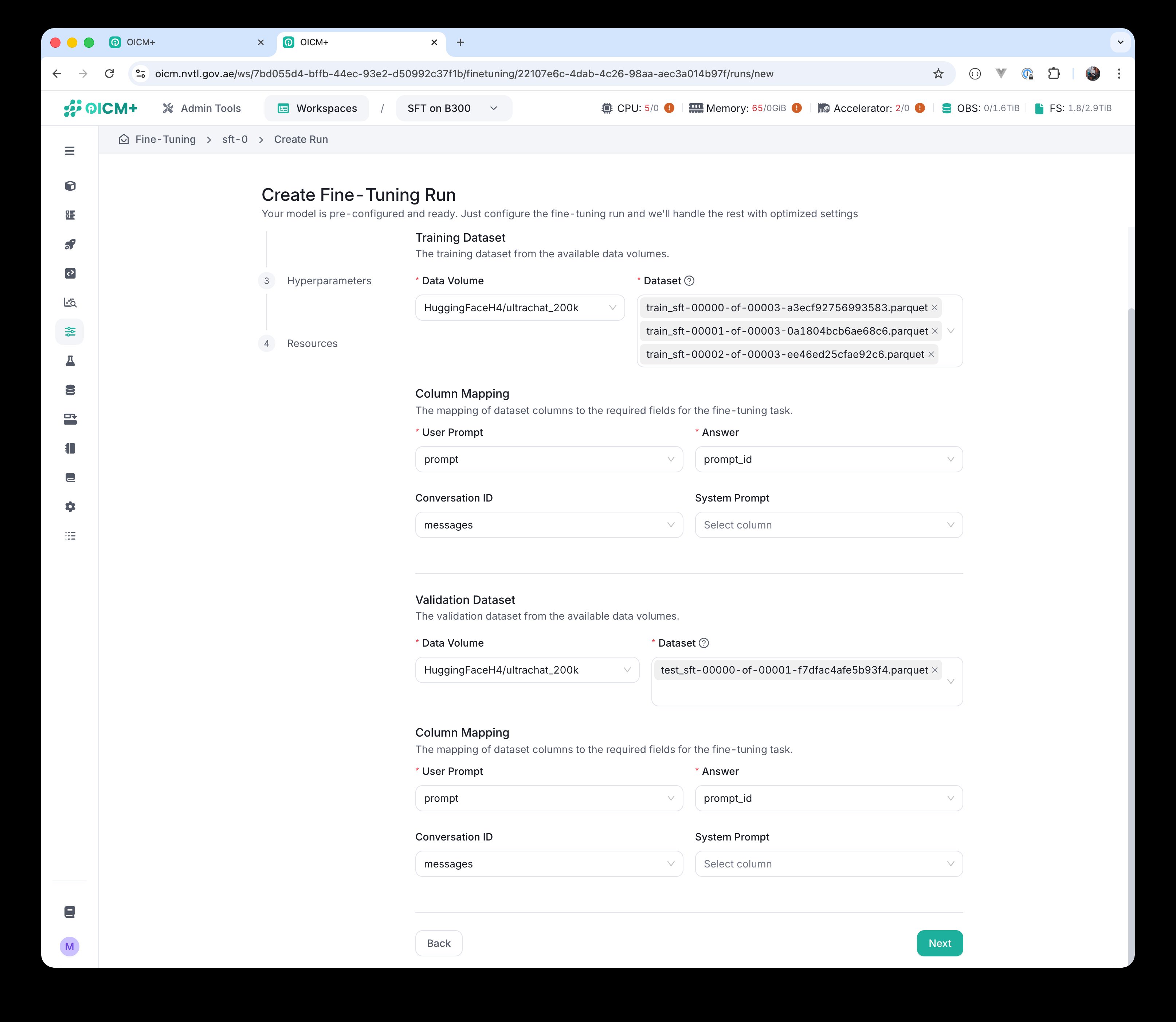 Step 2 with a real dataset —
 HuggingFaceH4/ultrachat_200k volume, parquet files selected, and columns mapped (prompt → User Prompt, prompt_id → Answer, messages → Conversation ID).
Note
Both training and validation data volumes — and the parquet (or other) files inside them — must be prepared upfront in the Data Volumes module.
Step 3 — Hyperparameters
Step 3 covers the fine-tuning strategy, the basic hyperparameters that you will typically tune from run to run, the advanced hyperparameters for fine-grained control, and the checkpoint policy.
Fine-Tuning Strategy
Choose between two strategies:
- Full Fine-Tuning (High Resource) — updates all model parameters during training. Suitable for maximum model adaptation but requires significantly more compute and memory.
- Parameter Efficient Tuning (Low Resource) — updates only a small set of additional parameters while the base model stays frozen. Significantly reduces compute and memory.
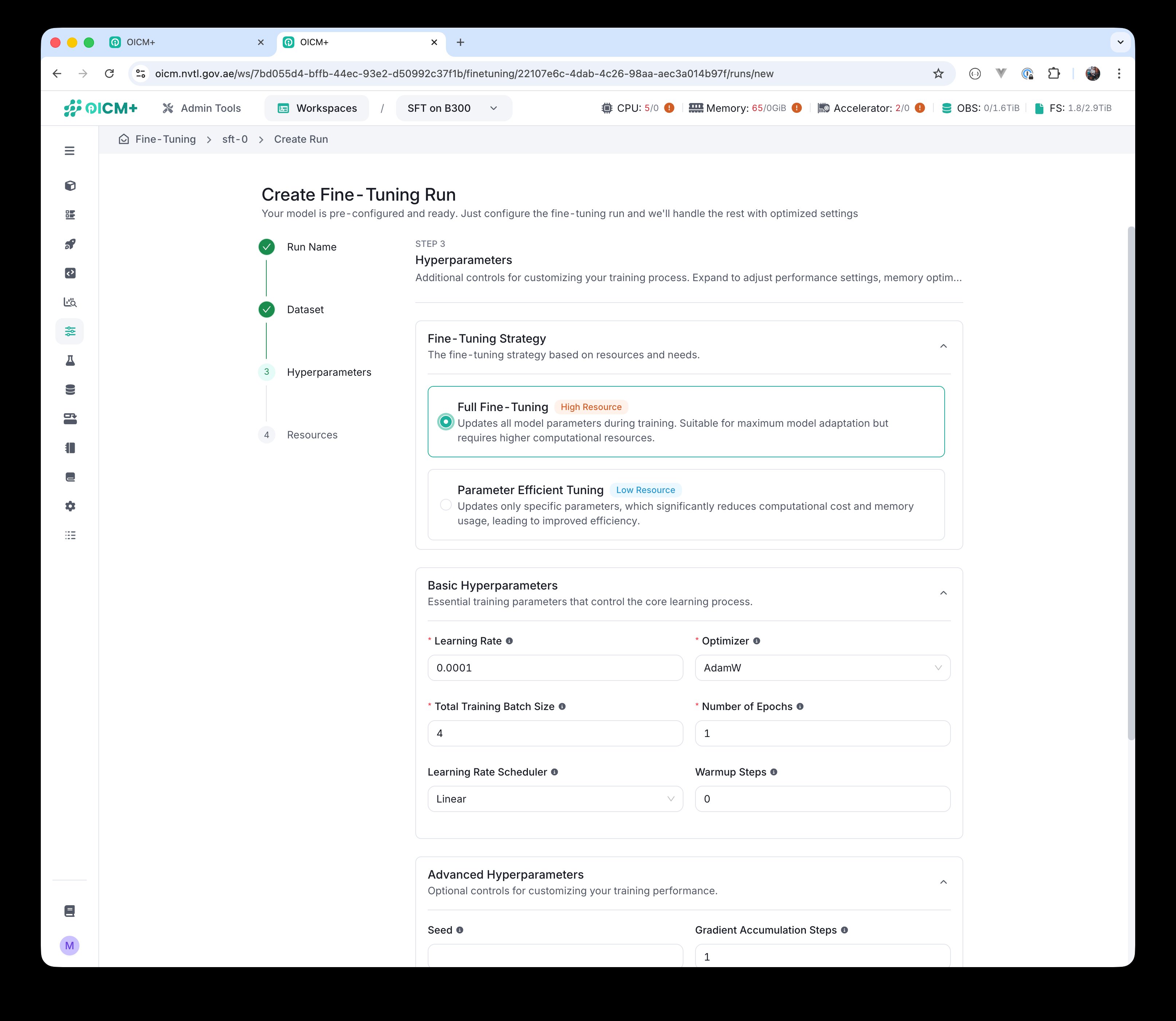 Step 3 — Fine-Tuning Strategy: Full Fine-Tuning selected.
If you select Parameter Efficient Tuning, a second choice appears underneath: LoRA, DoRA, or QLoRA (see section 3.3 for what each method does).
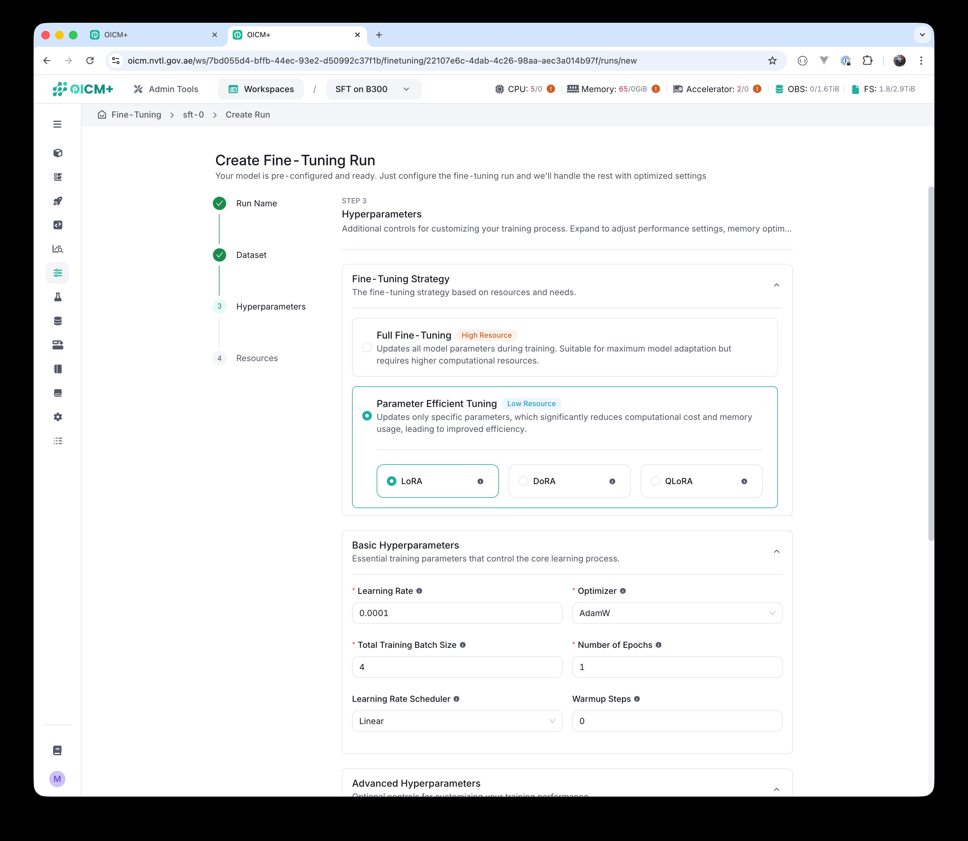 Parameter Efficient Tuning selected — pick one of LoRA, DoRA, or QLoRA.
Basic Hyperparameters
These are the essential parameters that control the core learning process. You will typically adjust them from run to run when iterating:
| Parameter | Default |
|---|---|
| Learning Rate | 0.0001 |
| Optimizer | AdamW |
| Total Training Batch Size | 4 |
| Number of Epochs | 1 |
| Learning Rate Scheduler | Linear |
| Warmup Steps | 0 |
Advanced Hyperparameters
These optional controls give experienced ML practitioners finer control over the training dynamics, regularization, and (for PEFT runs) adapter behavior. The defaults are sensible starting points and most users do not need to change them; adjust these only if you have a specific reason to.
| Parameter | Default | Notes |
|---|---|---|
| Seed | — | Random seed for reproducibility. |
| Gradient Accumulation Steps | 1 |
|
| Gradient Clipping | — | Caps gradient magnitude to prevent exploding gradients. |
| Regularization (Weight Decay) | 0.01 |
|
| Adapter Rank | 8 |
PEFT only. |
| Adapter Alpha | 16 |
PEFT only. |
| Adapter Dropout | 0.0 |
PEFT only. |
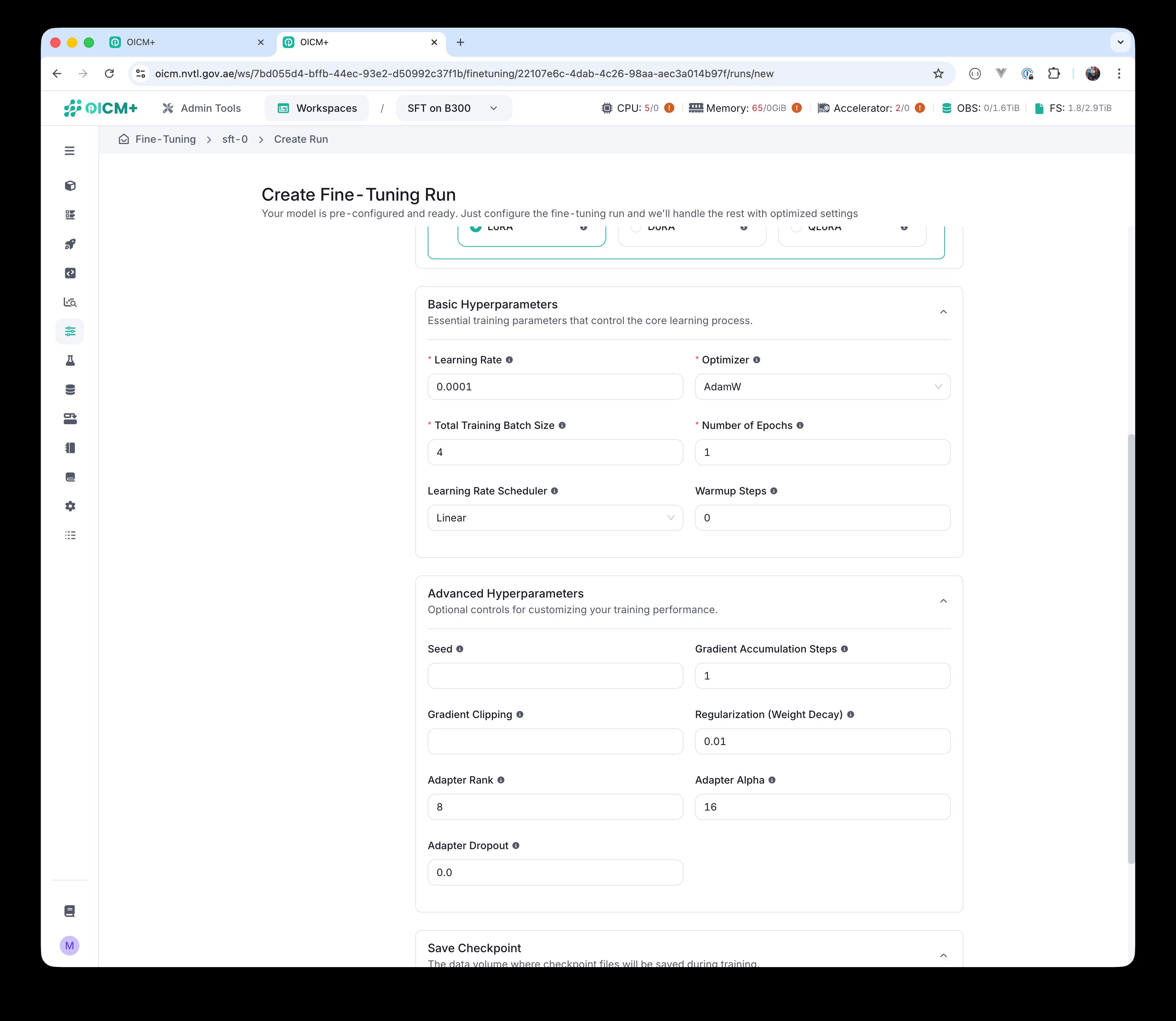 Step 3 — Advanced Hyperparameters section expanded.
Save Checkpoint
Choose where checkpoints are saved and how many to keep.
- Checkpoint FS Data Volume — the data volume where checkpoint files will be saved during training. This data volume must be created in advance in the Data Volumes module. Ideally this data volume should be empty, otherwise data may be overwritten and you might lose precious information.
- Checkpoint Strategy — how many checkpoints to keep. Three options:
- All — save every checkpoint. The number of stored checkpoints depends on the number of epochs and the validation frequency.
- Best — save only the checkpoint with the lowest validation loss.
- Latest — save only the latest checkpoint.
Note
Independent of the checkpointing strategy, the data volume will store recipe state, which takes up additional space. It is there to allow resuming the run from where it left off.
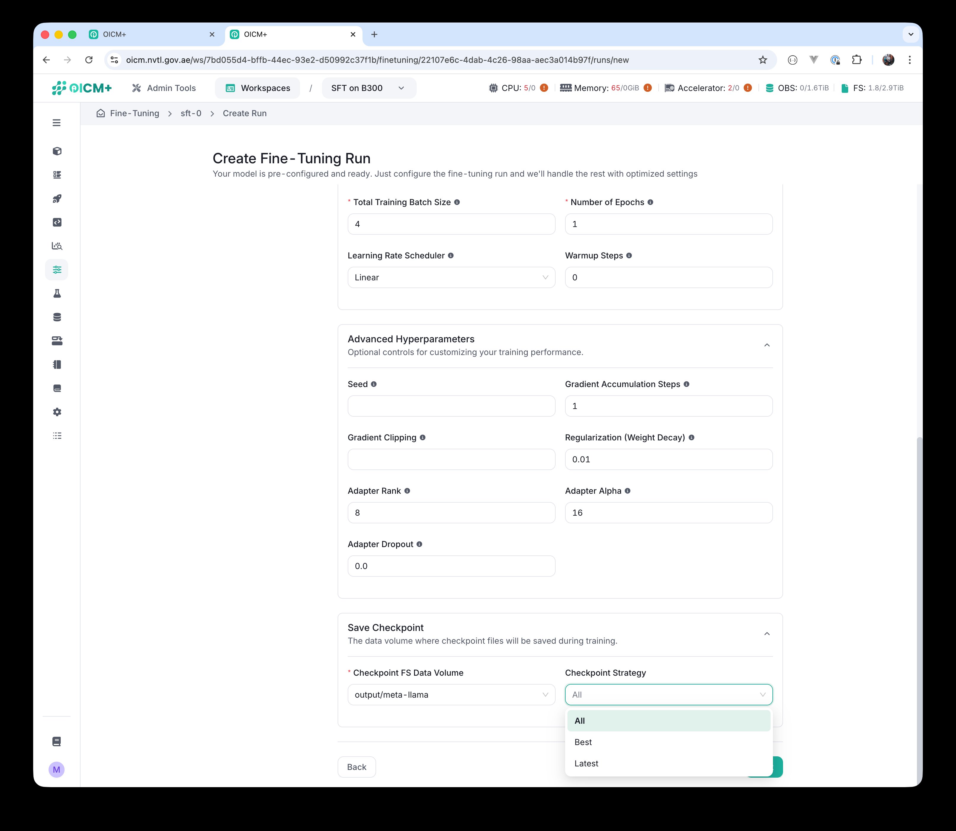 Save Checkpoint section — Checkpoint Strategy dropdown with All, Best, Latest.
Step 4 — Resources
Step 4 configures the compute resources for the run: which accelerator type to use, how many replicas to run on, and how much CPU, RAM and accelerator memory each replica gets.
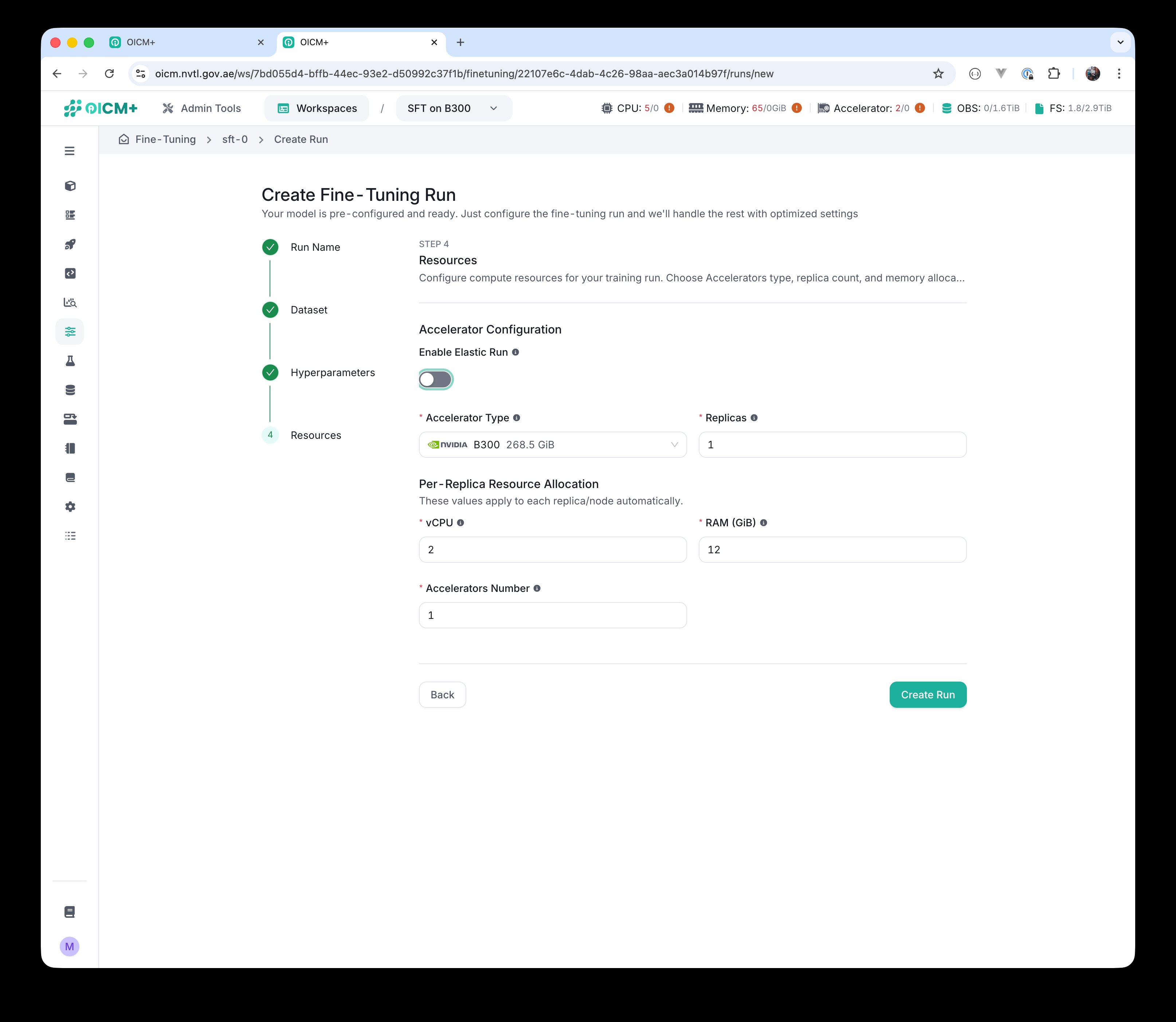
Accelerator Configuration
Choose your Accelerator Type from the available hardware. The Replicas field sets how many copies of the worker will run in parallel.
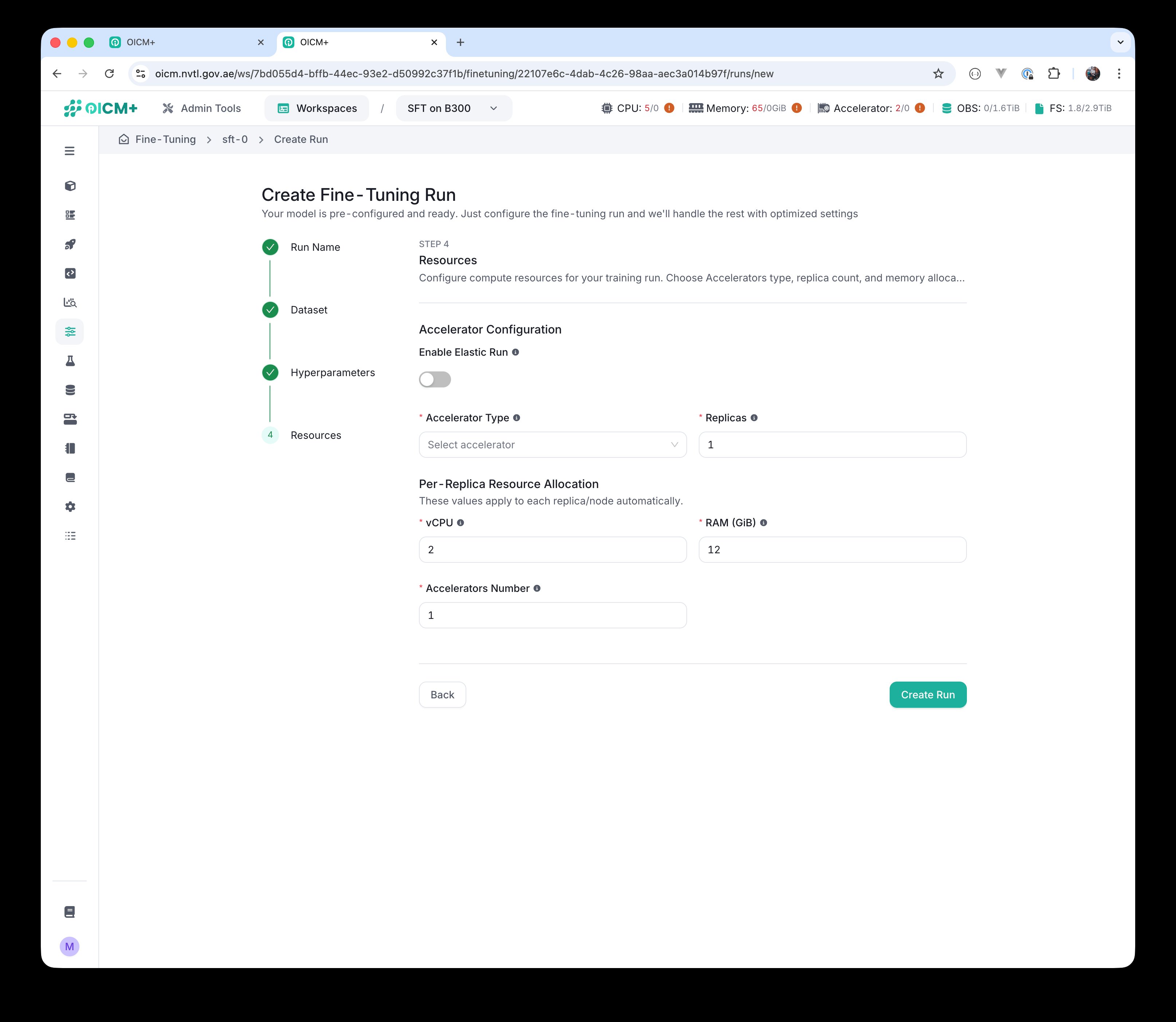 Step 4 — Resources with Elastic Run disabled. Single Replicas value.
Enable Elastic Run
Turning on Enable Elastic Run switches the resource model from a fixed replica count to a range. Instead of a single Replicas field you now specify Min Replicas, Max Replicas and Number of Restarts.
Note
Elastic Run is a resilience technique. You specify a minimum and a maximum number of replicas: if some worker nodes fail, the fine-tuning run automatically scales down (down to the minimum) and keeps making progress; when the failed nodes recover, it scales back up (up to the maximum) on its own. This avoids losing a long-running fine-tuning job to a transient node failure.
 Step 4 with Elastic Run enabled — Min Replicas, Max Replicas, and Number of Restarts replace the single Replicas field.
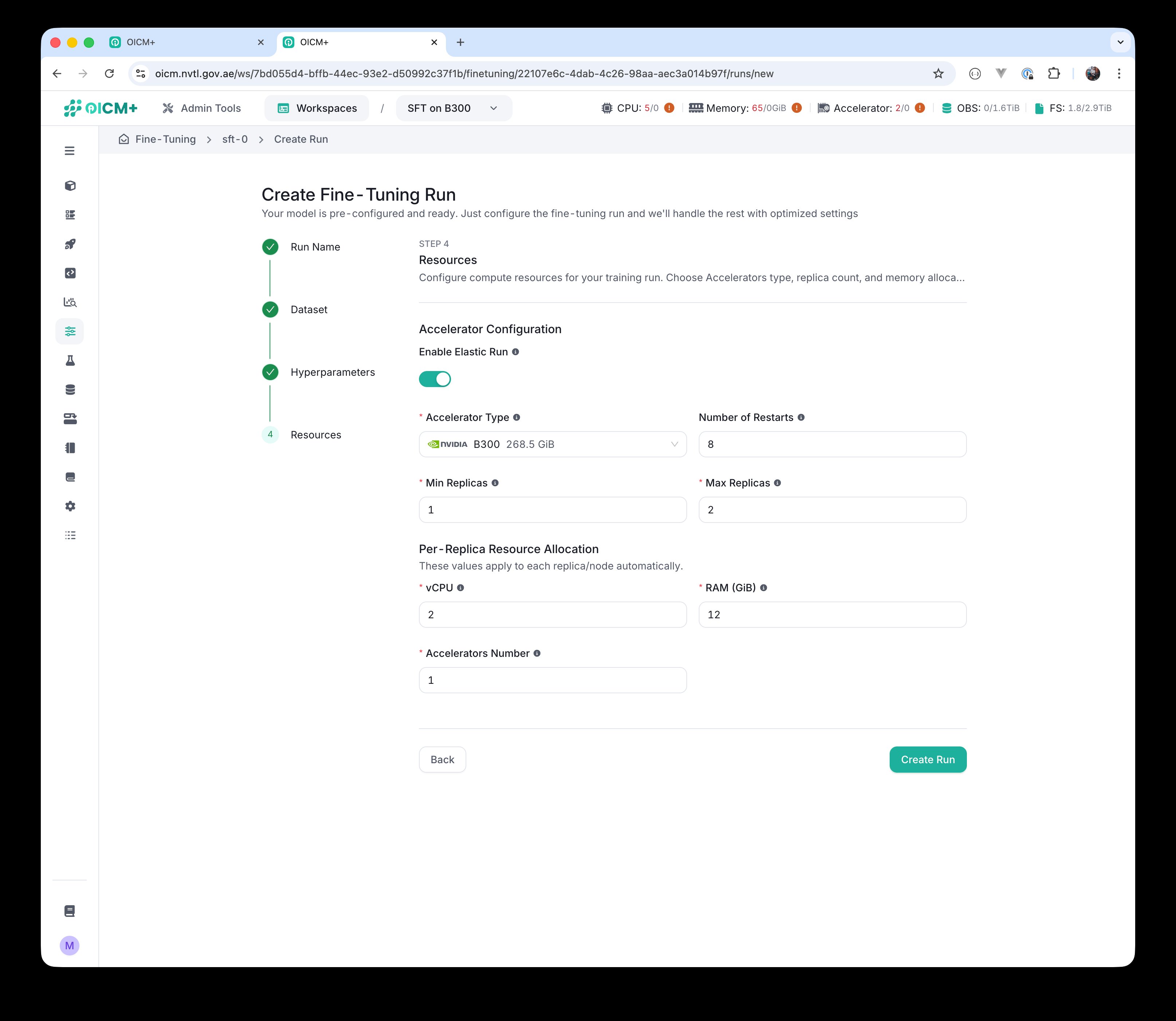 Elastic Run enabled with an accelerator selected.
Per-Replica Resource Allocation
These values apply to every replica/node automatically and let you size each worker:
| Parameter | Default |
|---|---|
| vCPU | 2 |
| RAM (GiB) | 12 |
| Accelerators Number | 1 |
Click Create Run at the bottom of step 4 to create the run.
Note
The relationship between replica count, accelerators per replica, and physical nodes may not be immediately intuitive. For example, if a node has 8 GPUs, you can deploy a single replica using all 8 GPUs or create 4 replicas with 2 GPUs each. Replica scheduling does not imply distribution across separate nodes — multiple replicas may still be scheduled onto the same physical node depending on resource availability.
4.3 The Created state — review and edit before launch
After clicking Create Run you are taken to the run page. The run is in the Created state — it is configured but has not been launched yet. A Configuration Preview card summarises the key choices (Dataset, Base Model, Output, Experiment, Task Type, Learning Rate, Batch Size) and a green Run button appears in the top right.
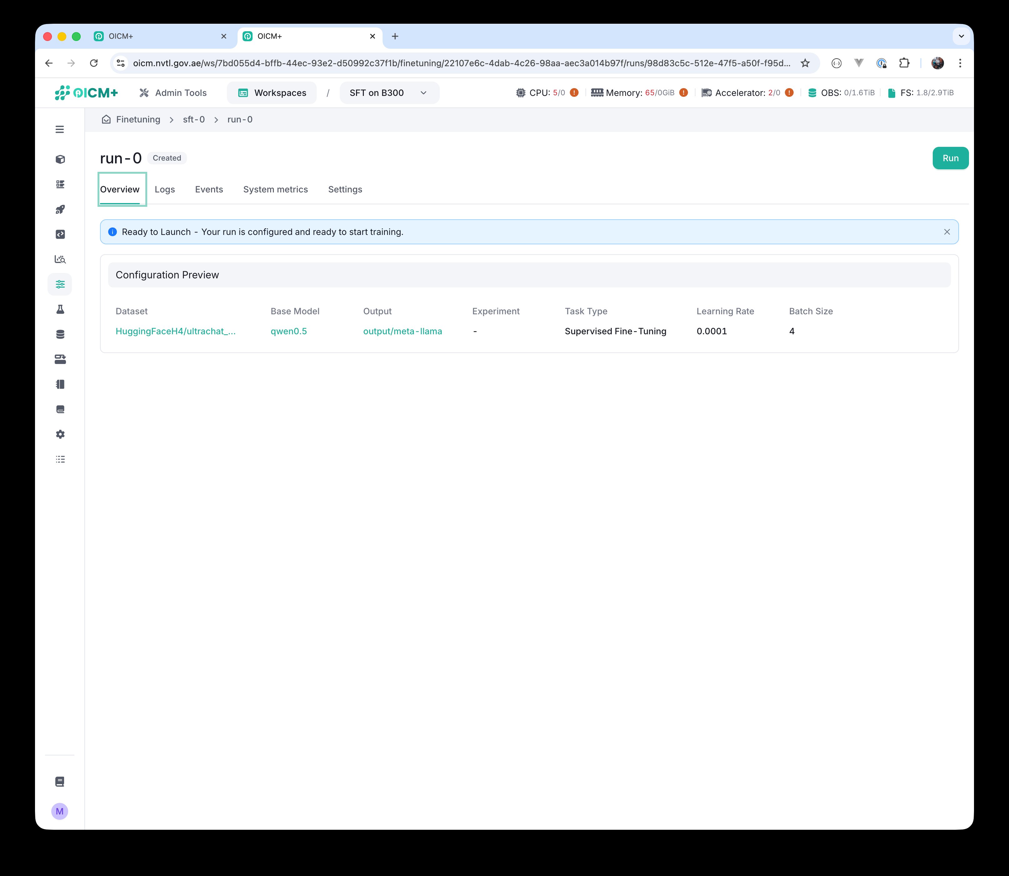 Run in Created state — Configuration Preview, plus the green Run button in the top right.
While the run is in the Created state you can still change any parameter you configured in the wizard. Open the Settings tab — every section from the four wizard steps is available as a collapsible block (Run Details, Datasets, Fine-Tuning Strategy, Basic Hyperparameters, Advanced Hyperparameters, Save Checkpoint, Resources). Make your changes and click Save Changes. The Delete button at the bottom of the Settings tab removes the run entirely.
When you are happy with the configuration, click the green Run button in the top right to launch the run. The run transitions from Created to an Active state (Initializing, Pending, Running). You can stop an Active run at any moment.
4.4 Monitor a running run
Once a run is launched, two additional views become available on the run page: Logs and System metrics.
Logs
The Logs tab streams the per-worker training output. You can jump to the Head (start) or Tail (latest) of the log, filter by Time range, search the text, and switch between the workers of a distributed run.
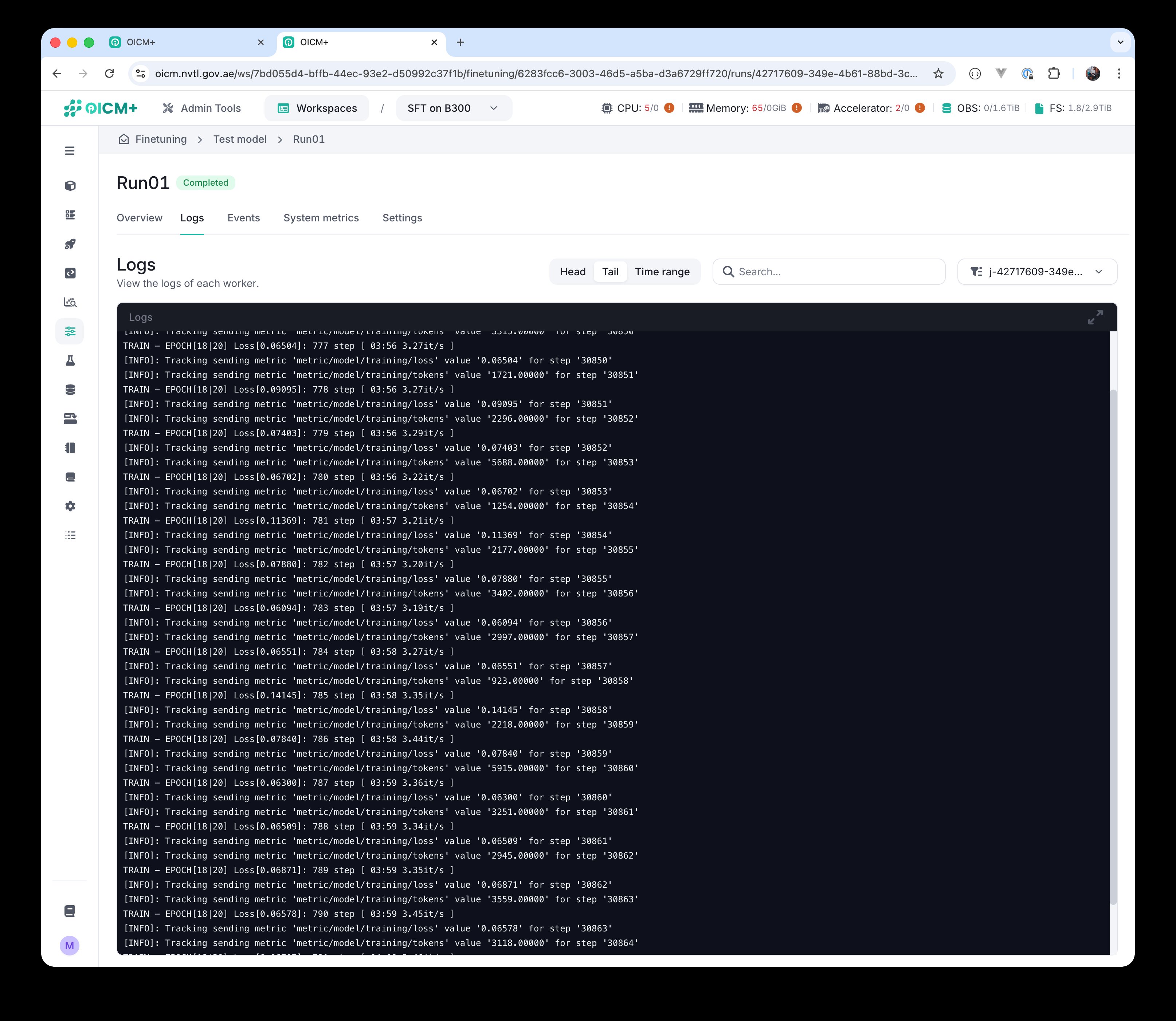 Logs tab — live training output with per-worker filtering.
System metrics
The System metrics tab shows real-time charts for each worker, with one line per replica:
- GPU Utilization — the percentage of GPU compute being used over time.
- GPU Temperature — current GPU temperature in degrees Celsius.
- Memory Utilization — how much GPU memory the run is currently using (in MiB).
- Power Draw — current power draw of the GPU in watts.
Encoder Utilization and Decoder Utilization are also reported and show video-engine usage (typically zero for LLM training).
 System metrics tab: GPU utilization, temperature, memory, encoder/decoder utilization, and power draw per worker.
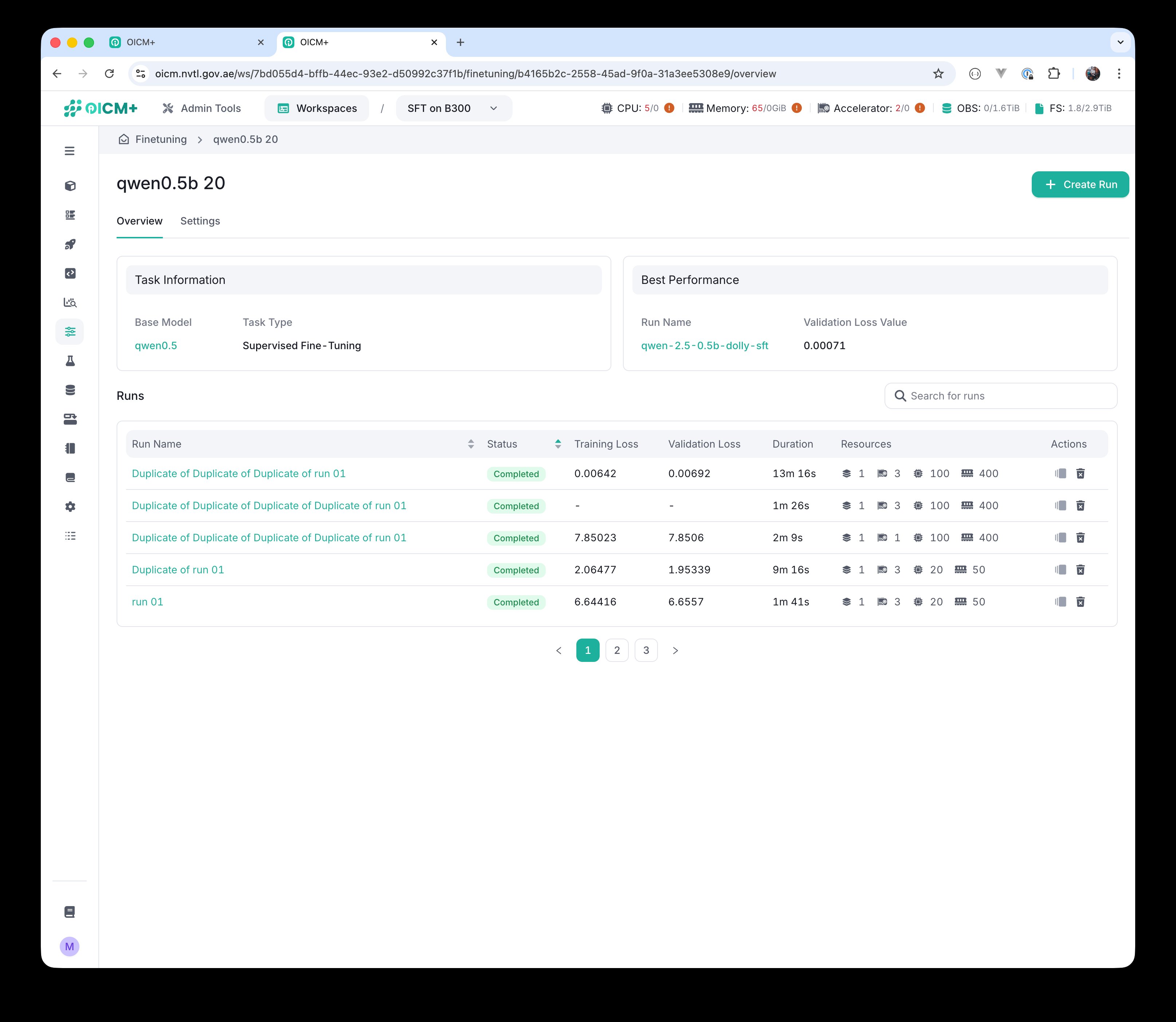
4.5 The task screen — comparing runs
In addition to per-run logs and metrics, the task screen lists every run created against the same task. Each row shows the run name, status, training loss, validation loss, duration, and the resources allocated to that run. For active runs, the training loss, validation loss, and duration values update close to real time.
 Task screen — list of runs with status, training loss, validation loss, duration, and resources for each.
Once a run completes, the Best Performance widget in the top-right of the task overview is updated automatically: it shows the run name and validation loss of the best-performing run on this task so far. This gives you a fast answer to "which of my runs should I consider for further analysis".
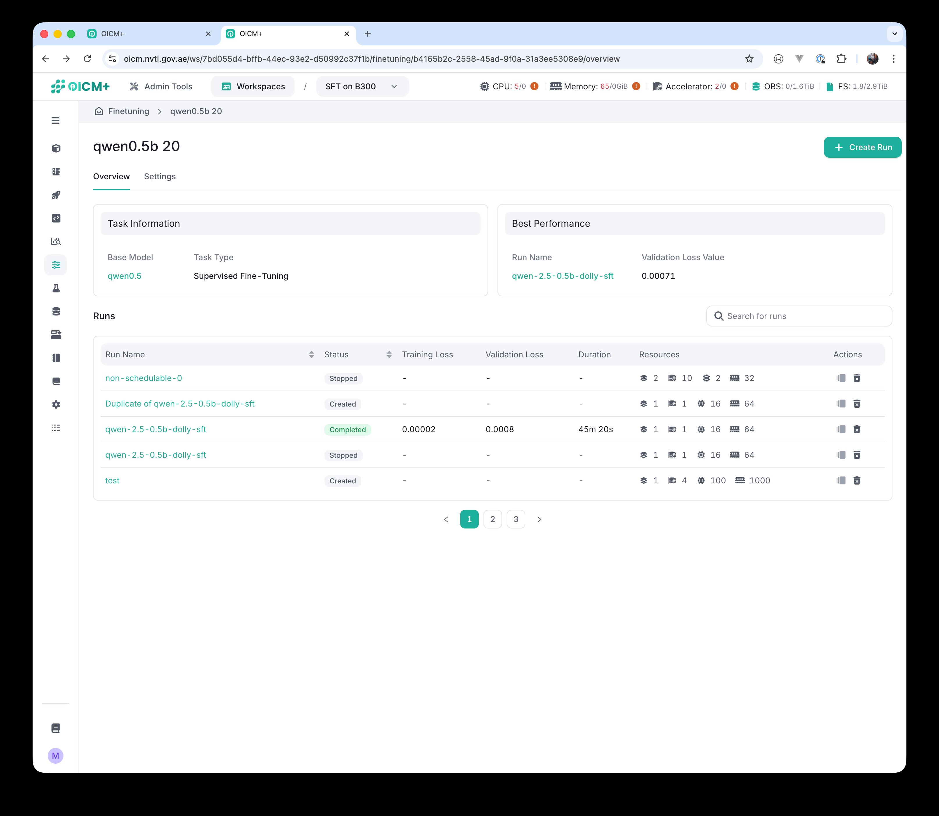 Task overview after multiple runs — Best Performance widget on the right shows the run with the lowest validation loss.
4.6 What to do with the resulting model
When a run completes, the resulting model is ready to be evaluated and compared against your baselines. Two paths typically follow:
- Benchmark it. Benchmarking can be done with a script after the model is deployed within OICM (or outside the platform) to compare it against the base model and against the model currently in production, on the metrics that matter for your use case. This step is what tells you whether the new model is actually an improvement.
- Deploy it in OICM. Hand the model off to the Deployment module to serve it.
4.7 Granular metrics in the Tracking module
Every fine-tuning run is linked to an experiment in the Tracking module. If you need more detail than the per-run System metrics tab provides — including training curves over steps, per-metric panels, and richer system telemetry — open the Tracking experiment that corresponds to the run.
Overview — run parameters and latest metrics
The Overview tab of a Tracking run lists every run parameter (type, strategy, epochs, batch size, optimizer, learning rate, gradient accumulation steps, …) on the left, and the latest metric values on the right and below. Run information (status, run id, created/updated timestamps, run duration) sits in a card on the right.
![]() Tracking — Overview tab with Run params, Run information, and Latest metrics.
Tracking — Overview tab with Run params, Run information, and Latest metrics.
Metrics — training and validation curves
The Metrics tab plots every tracked metric over the training steps. The default view includes:
metric/model/validation/loss— validation loss curve.metric/model/training/loss— training loss curve.metric/model/validation/tokens— validation tokens seen.metric/model/training/tokens— training tokens seen.
![]() Tracking — Metrics tab with validation and training loss curves, plus token counts.
Tracking — Metrics tab with validation and training loss curves, plus token counts.
System metrics — granular system telemetry
The same Metrics tab also includes a System Metrics section with finer-grained system telemetry than the per-run view:
system/system_memory_usage_percentageandsystem/system_memory_usage_megabytes.system/network_receive_megabytesandsystem/network_transmit_megabytes.system/disk_usage_percentage,system/disk_usage_megabytes, andsystem/disk_available_megabytes.system/cpu_utilization_percentage.
![]() Tracking — System metrics panels: system memory, network receive, disk usage percentage, and system memory in MB.
Tracking — System metrics panels: system memory, network receive, disk usage percentage, and system memory in MB.
![]() Tracking — additional system panels: disk usage and available disk in megabytes, CPU utilization, and network transmit.
Tracking — additional system panels: disk usage and available disk in megabytes, CPU utilization, and network transmit.
5. Next steps
- Deployment UI — deploy and serve your fine-tuned model.
References
- NVIDIA Technical Blog — Introducing DoRA, a High-Performing Alternative to LoRA for Fine-Tuning. https://developer.nvidia.com/blog/introducing-dora-a-high-performing-alternative-to-lora-for-fine-tuning/
- Liu et al., DoRA: Weight-Decomposed Low-Rank Adaptation, ICML 2024. https://arxiv.org/abs/2402.09353